Tensor-Based Sum-Product Networks: Part II

July 10, 2019

In this post, we arrive at the second stop on the road to tensor-based implementations of Sum-Product Networks. The code snippets in this post are also part of the implementation of LibSPN, although the library accomplishes all of it in a more generic way. Be sure to check out the library!

In Part I, we have looked at the first principles for Sum-Product Networks. If some of the things in the bullet list below still seem unclear, make your way through Part I before continuing here:

SPNs consist of leaf nodes, sum nodes and product nodes.
Leaf nodes correspond to indicators (discrete) or components (continuous) of single variables.
A scope is a set of variables.
A parent node obtains the union of the scopes of its children.
Leaf nodes have scopes of exactly one variable.
The scope of the root node contains all variables.
Children of sum nodes must have identical scopes to ensure completeness.
Children of product nodes must have pairwise disjoint scopes to ensure decomposability.
Decomposability and completeness are sufficient properties for validity.
A valid SPN computes an unnormalized probability.
A normalized valid SPN computes a normalized probability directly.

Now let’s see how we can implement the most important parts of an SPN’s forward pass in TensorFlow.

Layered Implementations

Thinking of neural architectures or SPN structures in terms of layers helps us to quickly summarize the layout of a model. From the high-level description of these layers, we can get a grasp of the complexity of the model and understand how it divides and conquers its inputs. In the realm of neural networks, layers serve as the de facto implementation strategy. In fact, most feedforward layers can be expressed with only a few operations.

Take, for instance, a dense layer with ReLU activations:

Y = \max\{XW, 0\}

Where $X$ is a matrix with dimensions [batch, num_in] and $W$ is a weight matrix with dimensions [num_in, num_out]. In TensorFlow, this is written as follows:

Y = tf.nn.relu(tf.matmul(X, W))

Such that the output Y is a matrix of shape [batch, num_out].

Other layer types like convolutional layers or recurrent layers will require slightly different views on the dimensions and internal operations. Nevertheless, they usually have

A leading batch dimension for the input tensors;
Some sort of dot product operations with weight vectors to compute activations of neurons.

Our aim is to come up with an SPN implementation close to this approach: if we manage to describe SPN layers in terms of a few operations to compute all sum or product operations for all nodes in a single layer (and for all samples in the batch), then we maximally exploit TensorFlow’s ability to launch these operations in parallel on GPUs! As opposed to MLPs, such an implementation presents some nontrivial challenges specific to SPNs which we’ll get to shortly.

In the remainder of this post we look at a generic tensor-based implementation of the most important components in SPNs:

A sum layer that computes all sums at a particular depth of the SPN;
A product layer that computes all products at a particular depth of the SPN.

Sum Layer

A sum layer in an SPN computes weighted sums, similar to a dense layer in an MLP. There are two noticable differences with weighted sums in dense layers and weighted sums in SPN layers:

SPN layers compute probabilities and should be implemented to operate in the log-domain to avoid numerical underflow;
A single sum in a sum layer of an SPN is connected to only a subset of the preceding layer, as it can only have children with identical scopes (the completeness property).

Matrix Multiplications In The Log Domain

The first issue mentioned above makes it seem impossible to use matrix multiplications or similar dot-product based operations to compute our sum layer’s outputs. We can’t use anything like tf.matmul or tf.tensordot as these functions operate in linear space.

That’s utterly sad news! GPUs simply shine at doing matrix multiplications. Are we doomed already? Let’s try to find out.

Let’s take a step back and assume that we only want to compute the log-probability of a single sum node. A minimal implementation in TensorFlow would at least contain:

# x_prime is a vector of log-prob inputs, while w_prime is a vector of log weights 
out = tf.reduce_logsumexp(x_prime + w_prime)

Where $\boldsymbol x'=\log(\boldsymbol x)$ and $\boldsymbol w'=\log(\boldsymbol w)$ . As we’re operating in the log-domain, the pairwise multiplication of $\boldsymbol x$ and $\boldsymbol w$ becomes a pairwise addition of the log-space correspondents $\boldsymbol x'$ and $\boldsymbol w'$ .

To sum up the pairwise multiplications in log-space, we use tf.reduce_logsumexp. This built-in TensorFlow function computes the following:

y' = \log \left( \sum_i \exp(x_i' + w_i') \right)

Where $y' = \log(y) = \log(\boldsymbol x^\top \boldsymbol w)$ . But here lies a danger: computing $\exp(x_i' + w_i')$ would already result in underflow. The remedy is to subtract a constant $c$ from each element of the result of $x_i'$ and $w_i'$ :

y' = c + \log \left( \sum_i \exp(x_i' + w_i' - c) \right)

Usually, $c$ is set to $\max(x_1' + w_1', x_2'+w_2', \ldots, x_N'+w_N')$ . In fact, this is already part of the implementation of tf.reduce_logsumexp.

Extracting The Dot Product

But wait, this doesn’t look anything like a dot product! Let’s do something about that.

If you look closely, the equation of tf.reduce_logsumexp above just changes from the log domain to the linear domain before doing the summation and finally goes back to the log domain. If we forget about numerical stability for a bit, we could also read it as follows:

y' = \log \left( \sum_i \exp(x_i') \cdot \exp(w_i') \right)

The inner part $\sum_i \exp(x_i') \cdot \exp(w_i')$ is just a dot product of two exponentialized vectors (i.e. they are transformed from the log-domain to the linear domain). But if this is a dot product, could we use matrix multiplications for sum layers after all?

A naively applied dot product (or matrix multiplication) wouldn’t take care of numerical stability, so that would be a dead end…

Dot Products Without Underflow

The constant $c$ above was subtracted to avoid underflow, such that at least the higher values of the pairwise addition would not become zero after applying $\exp$ . But do we have to sum up $x'_i$ and $w'_i$ before subtracting $c$ ? Why not subtract a constant $c$ from $\boldsymbol x'$ and another constant $d$ from $\boldsymbol w'$ directly?

y' = c + d + \log \left( \sum_i \exp(x_i' - c) \cdot \exp(w_i' - d) \right)

By doing so, we obtain a dot product while preserving numerical stability. Splendid!

Since matrix multiplications are just multiple dot products (where vectors are potentially reused in several dot products in the resulting matrix), we can generalize the trick above as follows:

Y' = C + D + \log\bigg( \exp\big(X'-C\big) \exp\big(W'-D\big) \bigg)

LibSPN implements a logmatmul function that uses this idea which is displayed here:

def logmatmul(a, b, transpose_a=False, transpose_b=False, name=None):
    with tf.name_scope(name, "logmatmul", [a, b]):
        # Number of outer dimensions
        num_outer_a = len(a.shape) - 2
        num_outer_b = len(b.shape) - 2

        # Reduction axis
        reduce_axis_a = num_outer_a if transpose_a else num_outer_a + 1
        reduce_axis_b = num_outer_b + 1 if transpose_b else num_outer_b

        # Compute max for each tensor for numerical stability
        max_a = replace_infs_with_zeros(
            tf.stop_gradient(tf.reduce_max(a, axis=reduce_axis_a, keepdims=True)))
        max_b = replace_infs_with_zeros(
            tf.stop_gradient(tf.reduce_max(b, axis=reduce_axis_b, keepdims=True)))

        # Subtract        a -= max_a        b -= max_b        # Compute logsumexp using matrix mutiplication        out = tf.log(tf.matmul(            tf.exp(a), tf.exp(b), transpose_a=transpose_a, transpose_b=transpose_b))
        # If necessary, transpose max_a or max_b
        if transpose_a:
            max_a = tf.transpose(
                max_a, list(range(num_outer_a)) + [num_outer_a + 1, num_outer_a])
        if transpose_b:
            max_b = tf.transpose(
                max_b, list(range(num_outer_b)) + [num_outer_b + 1, num_outer_b])
        out += max_a
        out += max_b
    return out

The highlighted block in the code above implements the matrix multiplication in the log domain with only a few operations. The remaining code is either to (i) determine the constants max_a and max_b or to (ii) know whether to transpose the inner-most dimensions of any of the inputs or (iii) to know which dimensions to use in case we have a so-called batched matrix multiplication with tensors of rank higher than 2. The replace_infs_with_zeros is to ensure that we don’t run into trouble when max_a or max_b contains -inf.

The matrix $X'$ corresponds to the log probabilities of the inputs of a set of sum nodes with the same scope. Each row in the matrix contains these inputs for a single sample in the batch. In other words, we could think of it as [batch, num_in_per_scope] dimensions.

The matrix $W'$ corresponds to the log weights of multiple sum nodes which are all connected to the same set of children with identical scopes. Its dimensions are [num_in_per_scope, num_out_per_scope].

With the matrix multiplication in log-space we would be able to compute the sums activation in the highlighted part of the SPN in Figure 1:

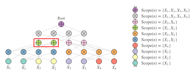
Figure 1: Sums with the same scope, such as the 2 nodes highlighted here, can be computed for all samples in the batch using a log-space matrix multiplication.

That’s good progress! This trick at least works for any number of inputs with the same scopes and any number of outputs. However, we are only computing a small part of the sum layer at the moment, so we’ll need to do better. We need to make it work for all scopes simultaneously.

Computing Sums For Multiple Scopes

Note that there’s a slight difference in the way we referred to the dimensions in the last paragraph as compared to MLPs. In the case of SPNs, we also care about scopes being identical for sum children. However, we want to do better than computing probabilities for a single scope only.

We can compute the weighted sums for all scopes at once by just introducing another dimension for the scopes in our tensors. That means that:

The input tensor X_prime will have a shape of [num_scopes, batch, num_in_per_scope]
The weight tensor W_prime will have a shape of [num_scopes, num_in_per_scope, num_out_per_scope].

Our implementation of logmatmul exploits the fact that tf.matmul is able to compute several matrix multiplications in parallel. In this case, they are parallelized over scopes. The docstrings of the matmul operation also list this example to clarify:

# 3-D tensor `a`
# [[[ 1,  2,  3],
#   [ 4,  5,  6]],
#  [[ 7,  8,  9],
#   [10, 11, 12]]]
a = tf.constant(np.arange(1, 13, dtype=np.int32),
                shape=[2, 2, 3])

# 3-D tensor `b`
# [[[13, 14],
#   [15, 16],
#   [17, 18]],
#  [[19, 20],
#   [21, 22],
#   [23, 24]]]
b = tf.constant(np.arange(13, 25, dtype=np.int32),
                shape=[2, 3, 2])

# `a` * `b`
# [[[ 94, 100],
#   [229, 244]],
#  [[508, 532],
#   [697, 730]]]
c = tf.matmul(a, b)

Note that the output tensor c is of shape [2, 2, 2], so there are 2 matrix multiplications performed in parallel. In the case of our tensorized SPNs, this would correspond to all sums in a layer for 2 different scopes.

This means that we can use logmatmul for computing the probabilities directly from X_prime and W_prime as it ‘batches’ the outer-most dimension (the one with num_scopes):

# X_prime.shape == [num_scopes, batch, num_in_per_scope]
# W_prime.shape == [num_scopes, num_in_per_scope, num_out_per_scope]
# Y_prime.shape == [num_scopes, batch, num_out_per_scope]

# The resulting tensor contains the log matrix multiplication for all scopes and
# for all sums per scope 
Y_prime = logmatmul(X_prime, W_prime)

Concise and super efficient!

Limitations Of This Approach

Although framing our forward pass this way is convenient and fast on GPUs, it also enforces us to have dimension sizes that are the same for any scope. In other words, each scope will have the same number of inputs and the same number of outputs, unless we explicitly mask these.

Nevertheless, the proposed approach maximally exploits CUDA’s GPU kernels for matrix multiplication. So even if we’d use separate matrix multplications for scopes with different dimensions instead of masking, the all-in-one Op approach is presumably still faster.

Product Layer

SPNs combine scopes by multiplying nodes. In other words, they compute joint probabilities by (hierarchically) multiplying probabilities of subsets of variables. Let’s say we have a sum layer for 2 scopes with 4 output nodes per scope. If we were to apply a product layer on top of this to join the two scopes, we can generate $4^2$ permutations of nodes. In general, if a product joins $m$ scopes of size $n$ each, there are $n^m$ possible permutations.

Let $\boldsymbol u$ be the vector of probabilities of the first scope and $\boldsymbol v$ be the vector of probabilities of the second scope. In that case, we can compute an outer product to find a matrix containing all possible permutations:

Y_{n,n} = \boldsymbol u \boldsymbol v^\top = \begin{pmatrix} u_1 v_1 & u_1 v_2 & \cdots & u_1 v_n \\ u_2 v_1 & u_2 v_2 & \cdots & u_2 v_n \\ \vdots & \vdots & \ddots & \vdots \\ u_n v_1 & u_n v_2 & \cdots & u_n v_n \end{pmatrix}

Rather than limiting ourselves to joining one pair of scopes for one sample, let’s try to do this for multiple pairs of scopes and any number of samples.

Suppose we have a tensor x of shape [num_scopes, batch, num_in]. We want to join pairs of adjacent scopes within this tensor by products. In linear space, we can achieve this as follows:

# The batch dimension is dynamic. Also assume we already have 
# int values for num_scopes and num_in
x_reshaped = tf.reshape(x, [num_scopes // 2, 2, -1, num_in])

# Split up this tensor to get two scopes with 'adjacent' scopes
u, v = tf.split(x, axis=1)

# Compute the outer product to join the scopes. Y will have 
# shape [num_scopes // 2, batch, num_in, num_in]
Y = tf.reshape(u, [num_scopes // 2, -1, num_in, 1]) * \ 
    tf.reshape(v, [num_scopes // 2, -1, 1, num_in])

# Flatten the matrix of permutations in a single axis
num_out = num_in * num_in
Y = tf.reshape(Y, [num_scopes // 2, -1, num_out])

TensorFlow will conveniently broadcast the values so that the outer product is computed for all scopes and all samples in the batch in one go. Broadcasting works with the addition operator too, so we can easily switch to log-space computation by just using + (rather than *).

Dummy Variables

With this approach we’re assuming that the number of scopes is divisible by 2. In general, if we stack product layers $\ell_1,\ell_2,\ldots,\ell_N$ , we need to have $\prod_i \phi_i$ scopes at the leaf layer where $\phi_i$ is the number of scopes being joined at product layer $\ell_i$ .

For example, if we want to stack 3 product layers that join e.g. 2, 4 and 2 scopes respectively, we’d have $2\cdot 4 \cdot 2=16$ scopes at the bottom-most layer. But if our data only has 15 different variables, then such a division of scopes doesn’t make sense.

There is a neat workaround for this. We can employ ‘dummy variables’ that are always marginalized out, such that they don’t affect computed inferences at all. We achieve this by setting the dummy variables to a fixed probability of 1, which just corresponds to zero-padding in log-space (since $\log 1 = 0$ ).

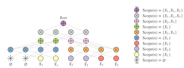
The SPN in Figure 2 below shows an example of dummy variables. Note that the two left-most leaf nodes have empty scopes, so that the blue product nodes on top of these only have $X_1$ in their scope.

Figure 2: An SPN with dummy variable indicators at the left-most leaf nodes. Such dummy indicators have empty scopes. In other words, they are always marginalized out.

Limitations And Extensions

There is no reason to limit ourselves to products that join just 2 scopes. We might as well perform outer products on the last $m > 2$ dimensions if we want to join any number of scopes. In that case, we would have to change the implementation of the product layer a little bit, but the general idea is the same.

One limitation of this approach is that we enforce the same number of outputs for all scopes in the SPN. So again, unless we mask inputs or outputs of these products somehow, our structure is forced to be homogeneous.

Adding Decompositions

In many cases, SPNs consist of several so-called decompositions. A decomposition describes how scopes are joined hierarchically from the leaf nodes all the way up to the root. The penultimate layer of the SPN in Figure 1 (with the grey product nodes under the root) decomposes $\{X_1,X_2,X_3\}$ into $\{X_1\}$ on the left side and $\{X_2,X_3\}$ on the right side. The bottom-most product layer decomposes $\{X_1\}$ into $\emptyset$ and $\{X_1\}$ at the blue product nodes and $\{X_2,X_3\}$ into $\{X_2\}$ and $\{X_3\}$ at the orange product nodes. We can summarize such a decomposition as:

\bigg\{\Big\{\emptyset,\{X_1\}\Big\},\Big\{\{X_2\},\{X_3\}\Big\}\bigg\}

But this decomposition is just one possibility. We can also have a decomposition such as the one in Figure 2:

Figure 3: An SPN with an alternative decomposition, easily achieved by just reordering the scopes at the leaf layer.

Which corresponds to:

\bigg\{\Big\{\emptyset,\{X_2\}\Big\},\Big\{\{X_1\},\{X_3\}\Big\}\bigg\}

Multiple Decompositions

In practice, SPNs often have more than 1 decomposition, so that different variable interactions and hierarchies can be modeled in different sub-SPNs. Most SPNs in the literature that are used for classification have a sub-SPN per class with a unique decomposition. Each class-specific sub-SPN has a root that contains all variables on top of the leaf nodes. Each of these class-specific roots can be joined by a root sum node.

Since multiple decompositions are so common in SPNs, the implementation of some types of sum layers and product layers in LibSPN use another leading dimension for decompositions (in addition to the scope dimension that we recently introduced). These particular layers compute sums or products for (i) all scopes, (ii) all decompositions and (iii) all samples in one go.

The internal tensors are represented as rank 4 tensors with dimensions [num_scopes, num_decompositions, batch, num_nodes_per_block]. In LibSPN, we refer to a pair of scope and decomposition as a block.

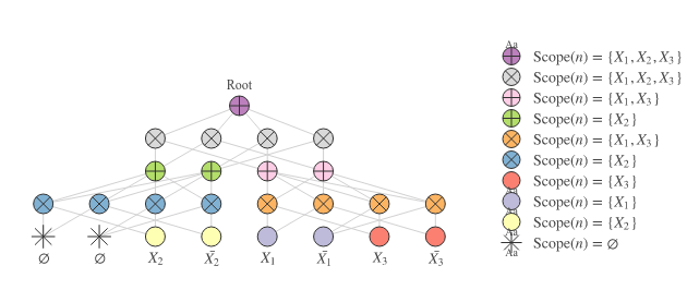
The following snippet constructs an SPN with a sum root and 2 sub-SPNs. The first sub-SPN corresponds to Figure 1 and the second to Figure 2 (note the fixed_permutations parameter).

import libspn as spn

# Layer with leaf indicators
indicators = spn.IndicatorLeaf(num_vars=3, num_vals=2)

# Layer that generates decompositions
x = spn.BlockGenerateDecompositions(
    indicators, num_decomps=2, 
    fixed_permutations=[[0, 1, 2], [1, 0, 2]]
)

# Permute nodes of two different scopes
x = spn.BlockPermuteProduct(x, num_factors=2)

# Two sums on top of each scope / decomposition
x = spn.BlockSum(x, num_sums_per_block=2)

# Permute nodes of two different scopes
x = spn.BlockPermuteProduct(x, num_factors=2)

# Merge the 2 decompositions into 1
x = spn.BlockMergeDecomps(x, num_decomps=1)

# Construct a root node
root = spn.BlockRootSum(x)

There you have it: tensor-based implementations of sum layers and product layers for building SPNs! There is still work to do to train such SPNs, but at least we got the most important elements in place now.

In the next post of this series, we’ll cover training of SPNs for generative or discriminative problems, so stay tuned!

Written by Jos van de Wolfshaar, a Machine Learning practitioner who's living and working in Amsterdam.

← Tensor-Based Sum-Product Networks: Part I