Semi-Supervised Learning With GANs

In this post I will cover a partial re-implementation of a recent paper on manifold regularization (Lecouat et al., 2018) for semi-supervised learning with Generative Adversarial Networks (Goodfellow et al., 2014). I will attempt to re-implement their main contribution, rather than getting all the hyperparameter details just right. Also, for the sake of demonstration, time constraints and simplicity, I will consider the MNIST dataset rather than the CIFAR10 or SVHN datasets as done in the paper. Ultimately, this post aims at bridging the gap between the theory and implementation for GANs in the semi-supervised learning setting. The code that comes with this post can be found here.

Generative Adversarial Networks

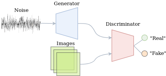
Let’s quickly go over Generative Adversarial Networks (GAN). In terms of the current pace within the AI/ML community, they have been around for a while (just about 4 years), so you might already be familiar with them. The ‘vanilla’ GAN procedure is to train a generator to generate images that are realistic and capable of fooling a discriminator. The generator generates the images by means of a deep neural network that takes in a noise vector $\boldsymbol z$.

The discriminator (which is a deep neural network as well) is fed with the generated images, but also with some real data. Its job is to say whether each image is either real (coming from the dataset) or fake (coming from the generator), which in terms of implementation comes down to binary classification. The image below summarizes the vanilla GAN setup.

Semi-Supervised learning

Semi-supervised learning problems concern a mix of labeled and unlabeled data. Leveraging the information in both the labeled and unlabeled data to eventually improve the performance on unseen labeled data is an interesting and more challenging problem than merely doing supervised learning on a large labeled dataset. In this case we might be limited to having only about 200 samples per class. So what should we do when only a small portion of the data is labeled?

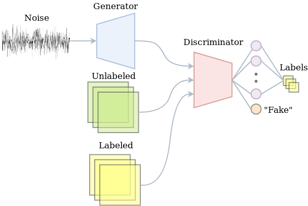
Note that adversarial training of vanilla GANs doesn’t require labeled data. At the same time, the deep neural network of the discriminator is able to learn powerful and robust abstractions of images by gradually becoming better at discriminating fake from real. Whatever it’s learning about unlabeled images will presumably also yield useful feature descriptors of labeled images. So how do we use the discriminator for both labeled and unlabeled data? Well, the discriminator is not necessarily limited to just telling fake from real. We could decide to train it to also classify the real data.

A GAN with a classifying discriminator would be able to exploit both the unlabeled as well as the labeled data. The unlabeled data will be used to merely tell fake from real. The labeled data would be used to optimize the classification performance. In practice, this just means that the discriminator has a softmax output distribution for which we minimize the cross-entropy. Indeed, part of the training procedure is just doing supervised learning. The other part is about adversarial training. The image below summarizes the semi-supervised learning setup with a GAN.

The Implementation

Let’s just head over to the implementation, since that might be the best way of understanding what’s happening. The snippet below prepares the data. It doesn’t really contain anything sophisticated. Basically, we take 400 samples per class and concatenate the resulting arrays as being our actual supervised subset. The unlabeled dataset consists of all train data (it also includes the labeled data, since we might as well use it anyway). As is customary for training GANs now, the output of the generator uses a hyperbolic tangent function, meaning its output is between $-1$ and $+1$. Therefore, we rescale the data to be in that range as well. Then, we create TensorFlow iterators so that we can efficiently go through the data later without having to struggle with feed dicts later on.

def prepare_input_pipeline(flags_obj):
    (train_x, train_y), (test_x, test_y) = tf.keras.datasets.mnist.load_data(
        "/home/jos/datasets/mnist/mnist.npz")

    def reshape_and_scale(x, img_shape=(-1, 28, 28, 1)):
        return x.reshape(img_shape).astype(np.float32) / 255. * 2.0 - 1.0

    # Reshape data and rescale to [-1, 1]
    train_x = reshape_and_scale(train_x)
    test_x = reshape_and_scale(test_x)

    # Shuffle train data
    train_x_unlabeled, train_y_unlabeled = shuffle(train_x, train_y)

    # Select subset as supervised
    train_x_labeled, train_y_labeled = [], []
    for i in range(flags_obj.num_classes):
        train_x_labeled.append(
            train_x_unlabeled[train_y_unlabeled == i][:flags_obj.num_labeled_examples])
        train_y_labeled.append(
            train_y_unlabeled[train_y_unlabeled == i][:flags_obj.num_labeled_examples])
    train_x_labeled = np.concatenate(train_x_labeled)
    train_y_labeled = np.concatenate(train_y_labeled)

    with tf.name_scope("InputPipeline"):

        def train_pipeline(data, shuffle_buffer_size):
            return tf.data.Dataset.from_tensor_slices(data)\
                .cache()\
                .shuffle(buffer_size=shuffle_buffer_size)\
                .batch(flags_obj.batch_size)\
                .repeat()\
                .make_one_shot_iterator()

        # Setup pipeline for labeled data
        train_ds_lab = train_pipeline(
            (train_x_labeled, train_y_labeled.astype(np.int64)),
            flags_obj.num_labeled_examples * flags_obj.num_classes)
        images_lab, labels_lab = train_ds_lab.get_next()

        # Setup pipeline for unlabeled data
        train_ds_unl = train_pipeline(
            (train_x_unlabeled, train_y_unlabeled.astype(np.int64)), len(train_x_labeled))
        images_unl, labels_unl = train_ds_unl.get_next()

        # Setup another pipeline that also uses the unlabeled data, so that we use a different
        # batch for computing the discriminator loss and the generator loss
        train_x_unlabeled, train_y_unlabeled = shuffle(train_x_unlabeled, train_y_unlabeled)
        train_ds_unl2 = train_pipeline(
            (train_x_unlabeled, train_y_unlabeled.astype(np.int64)), len(train_x_labeled))
        images_unl2, labels_unl2 = train_ds_unl2.get_next()

        # Setup pipeline for test data
        test_ds = tf.data.Dataset.from_tensor_slices((test_x, test_y.astype(np.int64)))\
            .cache()\
            .batch(flags_obj.batch_size)\
            .repeat()\
            .make_one_shot_iterator()
        images_test, labels_test = test_ds.get_next()

    return (images_lab, labels_lab), (images_unl, labels_unl), (images_unl2, labels_unl2), \
           (images_test, labels_test)

Next up is to define the discriminator network. I have deviated quite a bit from the architecture in the paper. I’m going to play safe here and just use Keras layers to construct the model. Actually, this enables us to very conveniently reuse all weights for different input tensors, which will prove to be useful later on. In short, the discriminator’s architecture uses 3 convolutions with $5\times 5$ kernels and strides of $2\times 2$, $2 \times 2$ and $1 \times 1$ respectively. Each convolution is followed by a leaky ReLU activation and a dropout layer with a dropout rate of 0.3. The flattened output of this stack of convolutions will be used as the feature layer.

The feature layer can be used for a feature matching loss (rather than a sigmoid cross-entropy loss as in vanilla GANs), which has proven to yield a more reliable training process. The part of the network up to this feature layer is defined in _define_tail in the snippet below. The _define_head method defines the rest of the network. The ‘head’ of the network introduces only one additional fully connected layer with 10 outputs, that correspond to the logits of the class labels. Other than that, there are some methods to make the interface of a Discriminator similar to that of tf.keras.models.Sequential.

class Discriminator:

    def __init__(self):
        """The discriminator network. Split up in a 'tail' and 'head' network, so that we can
        easily get the """
        self.tail = self._define_tail()
        self.head = self._define_head()

    def _define_tail(self, name="Discriminator"):
        """Defines the network until the intermediate layer that can be used for feature-matching
        loss."""
        feature_model = models.Sequential(name=name)

        def conv2d_dropout(filters, strides, index=0):
            # Adds a convolution followed by a Dropout layer
            suffix = str(index)
            feature_model.add(layers.Conv2D(
                filters=filters, strides=strides, name="Conv{}".format(suffix), padding='same',
                kernel_size=5, activation=tf.nn.leaky_relu))
            feature_model.add(layers.Dropout(name="Dropout{}".format(suffix), rate=0.3))

        # Three blocks of convs and dropouts. They all have 5x5 kernels, leaky ReLU and 0.3
        # dropout rate.
        conv2d_dropout(filters=32, strides=2, index=0)
        conv2d_dropout(filters=64, strides=2, index=1)
        conv2d_dropout(filters=64, strides=1, index=2)

        # Flatten it and build logits layer
        feature_model.add(layers.Flatten(name="Flatten"))
        return feature_model

    def _define_head(self):
        # Defines the remaining layers after the 'tail'
        head_model = models.Sequential(name="DiscriminatorHead")
        head_model.add(layers.Dense(units=10, activation=None, name="Logits"))
        return head_model

    @property
    def trainable_variables(self):
        # Return both tail's parameters a well as those of the head
        return self.tail.trainable_variables + self.head.trainable_variables

    def __call__(self, x, *args, **kwargs):
        # By adding this, the code below can treat a Discriminator instance as a
        # tf.keras.models.Sequential instance
        features = self.tail(x, *args, **kwargs)
        return self.head(features, *args, **kwargs), features

The generator’s architecture also uses $5 \times 5$ kernels. Many implementations of DCGAN-like architectures use transposed convolutions (sometimes wrongfully referred to as ‘deconvolutions’). I have decided to give the upsampling-convolution alternative a try. This should alleviate the issue of the checkerboard pattern that sometimes appears in generated images. Other than that, there are ReLU nonlinearities, and a first layer to go from the 100-dimensional noise to a (rather awkwardly shaped) $7 \times 7 \times 64$ spatial representation.

def define_generator():
    model = models.Sequential(name="Generator")

    def conv2d_block(filters, upsample=True, activation=tf.nn.relu, index=0):
        if upsample:
            model.add(layers.UpSampling2D(name="UpSampling" + str(index), size=(2, 2)))
        model.add(layers.Conv2D(
            filters=filters, kernel_size=5, padding='same', name="Conv2D" + str(index),
            activation=activation))

    # From flat noise to spatial
    model.add(layers.Dense(7 * 7 * 64, activation=tf.nn.relu, name="NoiseToSpatial"))
    model.add(layers.Reshape((7, 7, 64)))

    # Four blocks of convolutions, 2 that upsample and convolve, and 2 more that
    # just convolve
    conv2d_block(filters=128, upsample=True, index=0)
    conv2d_block(filters=64, upsample=True, index=1)
    conv2d_block(filters=64, upsample=False, index=2)
    conv2d_block(filters=1, upsample=False, activation=tf.nn.tanh, index=3)
    return model

I have tried to make this model work with what TensorFlow’s Keras layers have to offer so that the code would be easy to digest (and to implement of course). This also means that I have deviated from the architectures in the paper (e.g. I’m not using weight normalization). Because of this experimental approach, I have also experienced just how sensitive the training setup is to small variations in network architectures and parameters. There are plenty of neat GAN ‘hacks’ listed in this repo which I definitely found insightful.

Putting It Together

Let’s do the forward computations now so that we see how all of the above comes together. This consists of setting up the input pipeline, noise vector, generator and discriminator. The snippet below does all of this. Note that when define_generator returns the Sequential instance, we can just use it as a functor to obtain the output of it for the noise tensor given by $\boldsymbol z$.

The discriminator will do a lot more. It will take (i) the ‘fake’ images coming from the generator, (ii) a batch of unlabeled images and finally (iii) a batch of labeled images (both with and without dropout to also report the train accuracy). We can just repetitively call the Discriminator instance to build the graph for each of those outputs. Keras will make sure that the variables are reused in all cases. To turn off dropout for the labeled training data, we have to pass training=False explicitly.

(images_lab, labels_lab), (images_unl, labels_unl), (images_unl2, labels_unl2), \
            (images_test, labels_test) = prepare_input_pipeline(flags_obj)

with tf.name_scope("BatchSize"):
    batch_size_tensor = tf.shape(images_lab)[0]

# Get the noise vectors
z, z_perturbed = define_noise(batch_size_tensor, flags_obj)

# Generate images from noise vector
with tf.name_scope("Generator"):
    g_model = define_generator()
    images_fake = g_model(z)
    images_fake_perturbed = g_model(z_perturbed)

# Discriminate between real and fake, and try to classify the labeled data
with tf.name_scope("Discriminator") as discriminator_scope:
    d_model = Discriminator()
    logits_fake, features_fake          = d_model(images_fake, training=True)
    logits_fake_perturbed, _            = d_model(images_fake_perturbed, training=True)
    logits_real_unl, features_real_unl  = d_model(images_unl, training=True)
    logits_real_lab, features_real_lab  = d_model(images_lab, training=True)
    logits_train, _                     = d_model(images_lab, training=False)

The Discriminator’s Loss

Recall that the discriminator will be doing more than just separating fake from real. It also classifies the labeled data. For this, we define a supervised loss which takes the softmax output. In terms of implementation, this means that we feed the unnormalized logits to tf.nn.sparse_cross_entropy_with_logits.

Defining the loss for the unsupervised part is where things get a little bit more involved. Because the softmax distribution is overparameterized, we can fix the unnormalized logit at 0 for an image to be fake (i.e. coming from the generator). If we do so, the probability of it being real just turns into:

where $Z(x)$ is the sum of the unnormalized probabilities. Note that we currently only have the logits. Ultimately, we want to use the log-probability of the fake class to define our loss function. This can now be achieved by computing the whole expression in log-space:

Where the lower case $l$ with subscripts denote the individual logits. Divisions become subtractions and sums can be computed by the logsumexp function. Finally, we have used the definition of the softplus function:

In general, if you have the log-representation of a probability, it is numerically safer to keep things in log-space for as long as you can, since we are able to represent much smaller numbers in that case.

We’re not there yet. Generative adversarial training asks us to ascend the gradient of:

So whenever we call tf.train.AdamOptimizer.minimize we should descent:

Time to rewrite this a bit! The first term on the right-hand side of the equation can be written:

The second term of the right-hand side can be written as:

So that finally, we arrive at the following loss:

# Set the discriminator losses
with tf.name_scope("DiscriminatorLoss"):
    # Supervised loss, just cross-entropy. This normalizes p(y|x) where 1 <= y <= K
    loss_supervised = tf.reduce_mean(tf.nn.sparse_softmax_cross_entropy_with_logits(
        labels=labels_lab, logits=logits_real_lab))

    # Sum of unnormalized log probabilities
    logits_sum_real = tf.reduce_logsumexp(logits_real_unl, axis=1)
    logits_sum_fake = tf.reduce_logsumexp(logits_fake, axis=1)
    loss_unsupervised = 0.5 * (
        tf.negative(tf.reduce_mean(logits_sum_real)) +
        tf.reduce_mean(tf.nn.softplus(logits_sum_real)) +
        tf.reduce_mean(tf.nn.softplus(logits_sum_fake)))
    loss_d = loss_supervised + loss_unsupervised

Optimizing The Discriminator

Let’s set up the operations for actually updating the parameters of the discriminator. We will just reside to the Adam optimizer. While tweaking the parameters before I wrote this post, I figured I might slow down the discriminator by setting its learning rate at 0.1 times that of the generator. After that, my results got much better, so I decided to leave it there for now. Notice also that we can very easily select the subset of variables corresponding to the discriminator by exploiting the encapsulation offered by Keras.

# Configure discriminator training ops
with tf.name_scope("Train") as train_scope:
    optimizer = tf.train.AdamOptimizer(flags_obj.lr * 0.1)
    optimize_d = optimizer.minimize(loss_d, var_list=d_model.trainable_variables)
    train_accuracy_op = accuracy(logits_train, labels_lab)

Adding some control flow to the graph

After we have the new weights for the discriminator, we want the generator’s update to be aware of the updated weights. TensorFlow will not guarantee that the updated weights will actually be used even if we were to redeclare the forward computation after defining the minimization operations for the discriminator. We can still force this by using tf.control_dependencies. Any operation defined in the scope of this context manager will depend on the evaluation of the ones that are passed to context manager at instantiation. In other words, our generator’s update that we define later on will be guaranteed to compute the gradients using the updated weights of the discriminator.

with tf.name_scope(discriminator_scope):
    with tf.control_dependencies([optimize_d]):
        # Build a second time, so that new variables are used
        logits_fake, features_fake = d_model(images_fake, training=True)
        logits_real_unl, features_real_unl = d_model(images_unl2, training=True)

The Generator’s Loss And Updates

In this implementation, the generator tries to minimize the L2 distance of the average features of the generated images vs. the average features of the real images. This feature-matching loss (Salimans et al., 2016) has proven to be more stable for training GANs than directly trying to optimize the discriminator’s probability for observing real data. It is straightforward to implement. While we’re at it, let’s also define the update operations for the generator. Notice that the learning rate of this optimizer is 10 times that of the discriminator.

# Set the generator loss and the actual train op
with tf.name_scope("GeneratorLoss"):
    feature_mean_real = tf.reduce_mean(features_real_unl, axis=0)
    feature_mean_fake = tf.reduce_mean(features_fake, axis=0)
    # L1 distance of features is the loss for the generator
    loss_g = tf.reduce_mean(tf.abs(feature_mean_real - feature_mean_fake))

with tf.name_scope(train_scope):
    optimizer = tf.train.AdamOptimizer(flags_obj.lr, beta1=0.5)
    train_op = optimizer.minimize(loss_g, var_list=g_model.trainable_variables)

Adding manifold regularization

Lecouat et. al (2018) propose to add manifold regularization to the feature-matching GAN training procedure of Salimans et al. (2016). The regularization forces the discriminator to yield similar logits (unnormalized log probabilities) for nearby points in the latent space in which $\boldsymbol z$ resides. It can be implemented by generating a second perturbed version of $\boldsymbol z$ and computing the generator’s and discriminator’s outputs once more with this slightly altered vector.

This means that the noise generation code looks as follows:

def define_noise(batch_size_tensor, flags_obj):
    # Setup noise vector
    with tf.name_scope("LatentNoiseVector"):
        z = tfd.Normal(loc=0.0, scale=flags_obj.stddev).sample(
            sample_shape=(batch_size_tensor, flags_obj.z_dim_size))
        z_perturbed = z + tfd.Normal(loc=0.0, scale=flags_obj.stddev).sample(
            sample_shape=(batch_size_tensor, flags_obj.z_dim_size)) * 1e-5
    return z, z_perturbed

The discriminator’s loss will be updated as follows (note the 3 extra lines at the bottom):

# Set the discriminator losses
with tf.name_scope("DiscriminatorLoss"):
    # Supervised loss, just cross-entropy. This normalizes p(y|x) where 1 <= y <= K
    loss_supervised = tf.reduce_mean(tf.nn.sparse_softmax_cross_entropy_with_logits(
        labels=labels_lab, logits=logits_real_lab))

    # Sum of unnormalized log probabilities
    logits_sum_real = tf.reduce_logsumexp(logits_real_unl, axis=1)
    logits_sum_fake = tf.reduce_logsumexp(logits_fake, axis=1)
    loss_unsupervised = 0.5 * (
        tf.negative(tf.reduce_mean(logits_sum_real)) +
        tf.reduce_mean(tf.nn.softplus(logits_sum_real)) +
        tf.reduce_mean(tf.nn.softplus(logits_sum_fake)))
    loss_d = loss_supervised + loss_unsupervised
    if flags_obj.man_reg:        loss_d += 1e-3 * tf.nn.l2_loss(logits_fake - logits_fake_perturbed) \            / tf.to_float(batch_size_tensor)

Classification performance

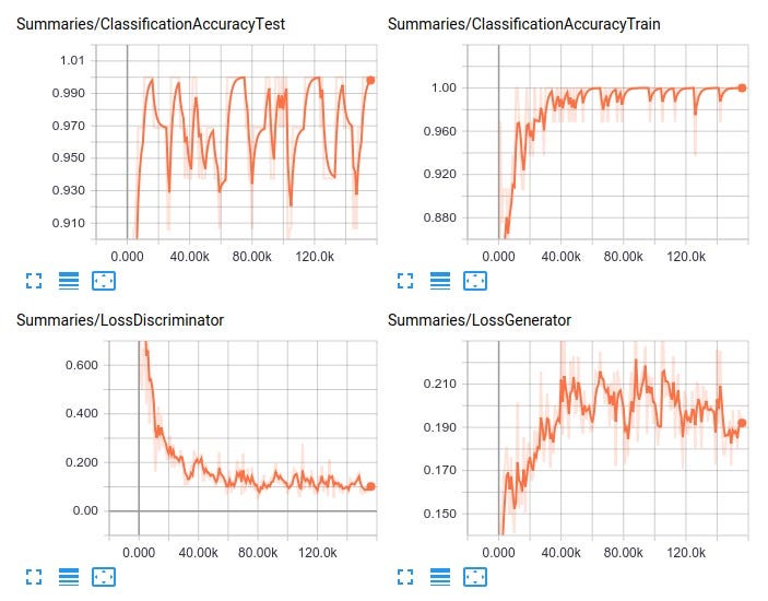
So how does it really perform? I have provided a few plots below. There are many things I might try to squeeze out additional performance (for instance, just training for longer, using a learning rate schedule, implementing weight normalization), but the main purpose of writing this post was to get to know a relatively simple yet powerful semi-supervised learning approach. After 100 epochs of training, the mean test accuracy approaches 98.9 percent.

The full script can be found in my repo. Thanks for reading!

Written by Jos van de Wolfshaar, a Machine Learning practitioner who's living and working in Amsterdam.